Training PyTorch ResNet in your TensorFlow Projects#

Framework Incompatibility#

Practitioners with large codebases written in other frameworks, such as PyTorch, are unable to take advantage of TensorFlow’s rich ecosystem of state-of-the-art (SOTA) deployment toolings, as this requires converting their code manually and inaccurately.

Ivy’s transpiler allows ML practitioners to dynamically connect libraries, layers and models from different frameworks together. For PyTorch users, the transpiler provides a seamless and accurate way to introduce code written in PyTorch to TensorFlow pipelines.

In this blog post, we’ll go through an example of how the transpiler can be used to convert a model from PyTorch to TensorFlow and train the converted model in TensorFlow.

Transpiling a PyTorch model to TensorFlow#

About the transpiled model#

To illustrate a typical transpilation workflow, we’ll be converting a pre-trained ResNet model from PyTorch to TensorFlow, and using the transpiled model to run inference.

ResNet owes its name to its residual blocks with skip connections that enable the model to be extremely deep. Even though including skip connections is a common idea in the community now, it was a revolutionary architectural choice and allowed ResNet to reach up to 152 layers with no vanishing or exploding gradient problems during training.

Architecturally, a ResNet block is similar to a ConvNext block but differs in terms of the specific convolutional layers used, grouped convolution, normalization, activation function, and downsampling. Going through the details of the models is outside the scope of this demo, interested readers might want to go through the paper.

Installation#

Since we want the packages to be available after installing, after running the first cell, the notebook will automatically restart.

You can then do Runtime -> Run all after the notebook has restarted, to run all of the cells.

Make sure you run this demo with GPU enabled!

[8]:

!pip install -q ivy

!python3 -m pip install torchvision
!python3 -m pip install astor

exit()

Requirement already satisfied: torchvision in /usr/local/lib/python3.10/dist-packages (0.18.0+cu121)
Requirement already satisfied: numpy in /usr/local/lib/python3.10/dist-packages (from torchvision) (1.25.2)
Requirement already satisfied: torch==2.3.0 in /usr/local/lib/python3.10/dist-packages (from torchvision) (2.3.0+cu121)
Requirement already satisfied: pillow!=8.3.*,>=5.3.0 in /usr/local/lib/python3.10/dist-packages (from torchvision) (9.4.0)
Requirement already satisfied: filelock in /usr/local/lib/python3.10/dist-packages (from torch==2.3.0->torchvision) (3.15.3)
Requirement already satisfied: typing-extensions>=4.8.0 in /usr/local/lib/python3.10/dist-packages (from torch==2.3.0->torchvision) (4.12.2)
Requirement already satisfied: sympy in /usr/local/lib/python3.10/dist-packages (from torch==2.3.0->torchvision) (1.12.1)
Requirement already satisfied: networkx in /usr/local/lib/python3.10/dist-packages (from torch==2.3.0->torchvision) (3.3)
Requirement already satisfied: jinja2 in /usr/local/lib/python3.10/dist-packages (from torch==2.3.0->torchvision) (3.1.4)
Requirement already satisfied: fsspec in /usr/local/lib/python3.10/dist-packages (from torch==2.3.0->torchvision) (2023.6.0)
Requirement already satisfied: nvidia-cuda-nvrtc-cu12==12.1.105 in /usr/local/lib/python3.10/dist-packages (from torch==2.3.0->torchvision) (12.1.105)
Requirement already satisfied: nvidia-cuda-runtime-cu12==12.1.105 in /usr/local/lib/python3.10/dist-packages (from torch==2.3.0->torchvision) (12.1.105)
Requirement already satisfied: nvidia-cuda-cupti-cu12==12.1.105 in /usr/local/lib/python3.10/dist-packages (from torch==2.3.0->torchvision) (12.1.105)
Requirement already satisfied: nvidia-cudnn-cu12==8.9.2.26 in /usr/local/lib/python3.10/dist-packages (from torch==2.3.0->torchvision) (8.9.2.26)
Requirement already satisfied: nvidia-cublas-cu12==12.1.3.1 in /usr/local/lib/python3.10/dist-packages (from torch==2.3.0->torchvision) (12.1.3.1)
Requirement already satisfied: nvidia-cufft-cu12==11.0.2.54 in /usr/local/lib/python3.10/dist-packages (from torch==2.3.0->torchvision) (11.0.2.54)
Requirement already satisfied: nvidia-curand-cu12==10.3.2.106 in /usr/local/lib/python3.10/dist-packages (from torch==2.3.0->torchvision) (10.3.2.106)
Requirement already satisfied: nvidia-cusolver-cu12==11.4.5.107 in /usr/local/lib/python3.10/dist-packages (from torch==2.3.0->torchvision) (11.4.5.107)
Requirement already satisfied: nvidia-cusparse-cu12==12.1.0.106 in /usr/local/lib/python3.10/dist-packages (from torch==2.3.0->torchvision) (12.1.0.106)
Requirement already satisfied: nvidia-nccl-cu12==2.20.5 in /usr/local/lib/python3.10/dist-packages (from torch==2.3.0->torchvision) (2.20.5)
Requirement already satisfied: nvidia-nvtx-cu12==12.1.105 in /usr/local/lib/python3.10/dist-packages (from torch==2.3.0->torchvision) (12.1.105)
Requirement already satisfied: triton==2.3.0 in /usr/local/lib/python3.10/dist-packages (from torch==2.3.0->torchvision) (2.3.0)
Requirement already satisfied: nvidia-nvjitlink-cu12 in /usr/local/lib/python3.10/dist-packages (from nvidia-cusolver-cu12==11.4.5.107->torch==2.3.0->torchvision) (12.5.40)
Requirement already satisfied: MarkupSafe>=2.0 in /usr/local/lib/python3.10/dist-packages (from jinja2->torch==2.3.0->torchvision) (2.1.5)
Requirement already satisfied: mpmath<1.4.0,>=1.1.0 in /usr/local/lib/python3.10/dist-packages (from sympy->torch==2.3.0->torchvision) (1.3.0)
Collecting astor
  Downloading astor-0.8.1-py2.py3-none-any.whl (27 kB)
Installing collected packages: astor
Successfully installed astor-0.8.1

Setting-up the source model#

We import the necessary libraries. We’ll mostly use the PyTorch’s Torchvision API to load the model, Ivy to transpile it from PyTorch to TensorFlow, and TensorFlow functions to fine-tune the transpiled model.

[1]:

import warnings
warnings.filterwarnings("ignore")
import logging
import tensorflow as tf
try:
   tf.config.experimental.set_memory_growth(
      tf.config.list_physical_devices("GPU")[0], True
   )
except:
   pass

# Filter TensorFlow info and warning messages
tf.get_logger().setLevel(logging.ERROR)
import os
import ivy
ivy.set_default_device("gpu:0")
import torch
import torchvision
from torchvision import datasets, models, transforms

torch.manual_seed(0)
tf.random.set_seed(0)

Load the Data#

We will use torchvision and torch.utils.data packages for loading the data.

The problem we’re going to solve today is to train a model to classify ants and bees. We have about 120 training images each for ants and bees. There are 75 validation images for each class. Usually, this is a very small dataset to generalize upon, if trained from scratch. Since we are using transfer learning, we should be able to generalize reasonably well.

This dataset is a very small subset of imagenet.

Note: Download the data from here and extract it to the current directory by running the following cell

[2]:

import requests
import os
import zipfile

# URL of the zip file you want to download
url = 'https://download.pytorch.org/tutorial/hymenoptera_data.zip'  # Replace with your URL

# Send a GET request to the URL
response = requests.get(url)

# Check if the request was successful (status code 200)
if response.status_code == 200:
    # Get the file name from the URL
    filename = os.path.basename(url)

    # Specify where you want to save the zip file (current working directory in Colab)
    zip_save_path = os.path.join(os.getcwd(), filename)

    # Write the content to the zip file
    with open(zip_save_path, 'wb') as f:
        f.write(response.content)

    print(f"Zip file downloaded successfully as '{filename}' in the current working directory.")

    # Extract the contents of the zip file
    with zipfile.ZipFile(zip_save_path, 'r') as zip_ref:
        zip_ref.extractall(os.getcwd())

    print("Zip file contents extracted successfully.")

    # Optionally, you can remove the zip file after extraction
    os.remove(zip_save_path)
    print(f"Zip file '{filename}' deleted.")

else:
    print(f"Failed to download zip file from '{url}'. Status code: {response.status_code}")

Zip file downloaded successfully as 'hymenoptera_data.zip' in the current working directory.
Zip file contents extracted successfully.
Zip file 'hymenoptera_data.zip' deleted.

[3]:

# Data augmentation and normalization for training
# Just normalization for validation
data_transforms = {
    'train': transforms.Compose([
        transforms.RandomResizedCrop(224),
        transforms.RandomHorizontalFlip(),
        transforms.ToTensor(),
        transforms.Normalize([0.485, 0.456, 0.406], [0.229, 0.224, 0.225])
    ]),
    'val': transforms.Compose([
        transforms.Resize(256),
        transforms.CenterCrop(224),
        transforms.ToTensor(),
        transforms.Normalize([0.485, 0.456, 0.406], [0.229, 0.224, 0.225])
    ]),
}

data_dir = 'hymenoptera_data'

image_datasets = {
    x: datasets.ImageFolder(
        os.path.join(data_dir, x), data_transforms[x]
    ) for x in ['train', 'val']
}

dataloaders = {
    x: torch.utils.data.DataLoader(
        image_datasets[x], batch_size=4,
        shuffle=True,
        num_workers=4
    ) for x in ['train', 'val']
}

dataset_sizes = {x: len(image_datasets[x]) for x in ['train', 'val']}
class_names = image_datasets['train'].classes
device = torch.device("cuda:0" if torch.cuda.is_available() else "cpu")

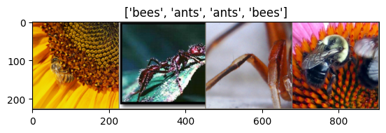
Visualize a few images#

We also load an input tensor to be passed as the input for transpilation

[4]:

import numpy as np
from matplotlib import pyplot as plt


def imshow(inp, title=None):
    """Display image for Tensor."""
    inp = inp.numpy().transpose((1, 2, 0))
    mean = np.array([0.485, 0.456, 0.406])
    std = np.array([0.229, 0.224, 0.225])
    inp = std * inp + mean
    inp = np.clip(inp, 0, 1)
    plt.imshow(inp)
    if title is not None:
        plt.title(title)
    plt.pause(0.001)  # pause a bit so that plots are updated


# Get a batch of training data
inputs, classes = next(iter(dataloaders['train']))

# Make a grid from batch
out = torchvision.utils.make_grid(inputs)

imshow(out, title=[class_names[x] for x in classes])

../../_images/demos_examples_and_demos_resnet_to_tensorflow_12_0.png

Load the pre-trained model#

We then initialise our ML model through the torchvision API, specifically we’ll be using ResNet18. Note that while we are using a model from the torchvision models API for this demonstration, it would still work with any arbitrary PyTorch model regardless of how it is being loaded. You can load models hosted on different platforms including local models.

[5]:

model = torchvision.models.resnet18(weights='IMAGENET1K_V1')
model

[5]:

ResNet(
  (conv1): Conv2d(3, 64, kernel_size=(7, 7), stride=(2, 2), padding=(3, 3), bias=False)
  (bn1): BatchNorm2d(64, eps=1e-05, momentum=0.1, affine=True, track_running_stats=True)
  (relu): ReLU(inplace=True)
  (maxpool): MaxPool2d(kernel_size=3, stride=2, padding=1, dilation=1, ceil_mode=False)
  (layer1): Sequential(
    (0): BasicBlock(
      (conv1): Conv2d(64, 64, kernel_size=(3, 3), stride=(1, 1), padding=(1, 1), bias=False)
      (bn1): BatchNorm2d(64, eps=1e-05, momentum=0.1, affine=True, track_running_stats=True)
      (relu): ReLU(inplace=True)
      (conv2): Conv2d(64, 64, kernel_size=(3, 3), stride=(1, 1), padding=(1, 1), bias=False)
      (bn2): BatchNorm2d(64, eps=1e-05, momentum=0.1, affine=True, track_running_stats=True)
    )
    (1): BasicBlock(
      (conv1): Conv2d(64, 64, kernel_size=(3, 3), stride=(1, 1), padding=(1, 1), bias=False)
      (bn1): BatchNorm2d(64, eps=1e-05, momentum=0.1, affine=True, track_running_stats=True)
      (relu): ReLU(inplace=True)
      (conv2): Conv2d(64, 64, kernel_size=(3, 3), stride=(1, 1), padding=(1, 1), bias=False)
      (bn2): BatchNorm2d(64, eps=1e-05, momentum=0.1, affine=True, track_running_stats=True)
    )
  )
  (layer2): Sequential(
    (0): BasicBlock(
      (conv1): Conv2d(64, 128, kernel_size=(3, 3), stride=(2, 2), padding=(1, 1), bias=False)
      (bn1): BatchNorm2d(128, eps=1e-05, momentum=0.1, affine=True, track_running_stats=True)
      (relu): ReLU(inplace=True)
      (conv2): Conv2d(128, 128, kernel_size=(3, 3), stride=(1, 1), padding=(1, 1), bias=False)
      (bn2): BatchNorm2d(128, eps=1e-05, momentum=0.1, affine=True, track_running_stats=True)
      (downsample): Sequential(
        (0): Conv2d(64, 128, kernel_size=(1, 1), stride=(2, 2), bias=False)
        (1): BatchNorm2d(128, eps=1e-05, momentum=0.1, affine=True, track_running_stats=True)
      )
    )
    (1): BasicBlock(
      (conv1): Conv2d(128, 128, kernel_size=(3, 3), stride=(1, 1), padding=(1, 1), bias=False)
      (bn1): BatchNorm2d(128, eps=1e-05, momentum=0.1, affine=True, track_running_stats=True)
      (relu): ReLU(inplace=True)
      (conv2): Conv2d(128, 128, kernel_size=(3, 3), stride=(1, 1), padding=(1, 1), bias=False)
      (bn2): BatchNorm2d(128, eps=1e-05, momentum=0.1, affine=True, track_running_stats=True)
    )
  )
  (layer3): Sequential(
    (0): BasicBlock(
      (conv1): Conv2d(128, 256, kernel_size=(3, 3), stride=(2, 2), padding=(1, 1), bias=False)
      (bn1): BatchNorm2d(256, eps=1e-05, momentum=0.1, affine=True, track_running_stats=True)
      (relu): ReLU(inplace=True)
      (conv2): Conv2d(256, 256, kernel_size=(3, 3), stride=(1, 1), padding=(1, 1), bias=False)
      (bn2): BatchNorm2d(256, eps=1e-05, momentum=0.1, affine=True, track_running_stats=True)
      (downsample): Sequential(
        (0): Conv2d(128, 256, kernel_size=(1, 1), stride=(2, 2), bias=False)
        (1): BatchNorm2d(256, eps=1e-05, momentum=0.1, affine=True, track_running_stats=True)
      )
    )
    (1): BasicBlock(
      (conv1): Conv2d(256, 256, kernel_size=(3, 3), stride=(1, 1), padding=(1, 1), bias=False)
      (bn1): BatchNorm2d(256, eps=1e-05, momentum=0.1, affine=True, track_running_stats=True)
      (relu): ReLU(inplace=True)
      (conv2): Conv2d(256, 256, kernel_size=(3, 3), stride=(1, 1), padding=(1, 1), bias=False)
      (bn2): BatchNorm2d(256, eps=1e-05, momentum=0.1, affine=True, track_running_stats=True)
    )
  )
  (layer4): Sequential(
    (0): BasicBlock(
      (conv1): Conv2d(256, 512, kernel_size=(3, 3), stride=(2, 2), padding=(1, 1), bias=False)
      (bn1): BatchNorm2d(512, eps=1e-05, momentum=0.1, affine=True, track_running_stats=True)
      (relu): ReLU(inplace=True)
      (conv2): Conv2d(512, 512, kernel_size=(3, 3), stride=(1, 1), padding=(1, 1), bias=False)
      (bn2): BatchNorm2d(512, eps=1e-05, momentum=0.1, affine=True, track_running_stats=True)
      (downsample): Sequential(
        (0): Conv2d(256, 512, kernel_size=(1, 1), stride=(2, 2), bias=False)
        (1): BatchNorm2d(512, eps=1e-05, momentum=0.1, affine=True, track_running_stats=True)
      )
    )
    (1): BasicBlock(
      (conv1): Conv2d(512, 512, kernel_size=(3, 3), stride=(1, 1), padding=(1, 1), bias=False)
      (bn1): BatchNorm2d(512, eps=1e-05, momentum=0.1, affine=True, track_running_stats=True)
      (relu): ReLU(inplace=True)
      (conv2): Conv2d(512, 512, kernel_size=(3, 3), stride=(1, 1), padding=(1, 1), bias=False)
      (bn2): BatchNorm2d(512, eps=1e-05, momentum=0.1, affine=True, track_running_stats=True)
    )
  )
  (avgpool): AdaptiveAvgPool2d(output_size=(1, 1))
  (fc): Linear(in_features=512, out_features=1000, bias=True)
)

Converting the model from TensorFlow to PyTorch#

With the model loaded, we can run the transpilation to TensorFlow eagerly. As we explain in our docs, eager transpilation involves manually providing dummy input arguments (tf.ones(4, 3, 224, 224) in our example) to use when tracing computational graphs.

[6]:

transpiled_model = ivy.transpile(model, source="torch", to="tensorflow", args=(inputs,))

WARNING:root:Native Numpy does not support GPU placement, consider using Jax instead

The transpiled graph can be used with any deep learning framework as backend and, in this case, adding the to='tensorflow' flag sets TensorFlow as the backend framework to use, thereby effectively converting the original PyTorch computational graph into a TensorFlow graph!

Comparing the results#

Let’s now try predicting the logits of the same input with the transpiled model

To compare the logits produced by the original and transpiled models at a more granular level, let’s try an allclose

[7]:

model.eval()
logits = model(inputs)
logits_np = logits.detach().numpy()

logits_transpiled = transpiled_model(tf.convert_to_tensor(inputs.numpy()), training=False)
logits_transpiled_np = logits_transpiled.numpy()

np.allclose(logits_np, logits_transpiled_np, atol=1e-4)

[7]:

True

The logits produced by the transpiled model at inference time are close to the ones produced by the original model, the logits are indeed consistent!

Fine-tuning the transpiled model#

One of the key benefits of using ivy’s transpiler is that the transpiled model is also trainable. As a result, we can also further train the transpiled model if required. Here’s an example of fine-tuning the transpiled model with a few images sampled from ImageNet using TensorFlow.

Let’s start by writing a general function to train a model.

[8]:

import time
import tensorflow as tf


def train_model(model, epochs, train_dataset, val_dataset, optimizer, loss_fn):
    # Prepare the metrics.
    train_acc_metric = tf.keras.metrics.SparseCategoricalAccuracy()
    val_acc_metric = tf.keras.metrics.SparseCategoricalAccuracy()

    for epoch in range(epochs):
        print("\nStart of epoch %d" % (epoch,))
        start_time = time.time()

        # Iterate over the batches of the dataset.
        for step, (x_batch_train, y_batch_train) in enumerate(train_dataset):

            x_batch_train = tf.convert_to_tensor(x_batch_train.detach().numpy())
            y_batch_train = tf.convert_to_tensor(y_batch_train.detach().numpy())

            with tf.GradientTape() as tape:
                logits = model(x_batch_train, training=True)
                loss_value = loss_fn(y_batch_train, logits)

            grads = tape.gradient(loss_value, model.trainable_weights)
            optimizer.apply_gradients(zip(grads, model.trainable_weights))

            # Update training metric.
            train_acc_metric.update_state(y_batch_train, logits)

            # Log every 20 batches.
            if step % 20 == 0:
                print(
                    "Training loss (for one batch) at step %d: %.4f"
                    % (step, float(loss_value))
                )
                print("Seen so far: %d samples" % ((step + 1) * 4))

        # Display metrics at the end of each epoch.
        train_acc = train_acc_metric.result()
        print("Training acc over epoch: %.4f" % (float(train_acc),))

        # Reset training metrics at the end of each epoch
        train_acc_metric.reset_states()

        # Run a validation loop at the end of each epoch.
        for x_batch_val, y_batch_val in val_dataset:
            x_batch_val = tf.convert_to_tensor(x_batch_val.detach().numpy())
            y_batch_val = tf.convert_to_tensor(y_batch_val.detach().numpy())

            val_logits = model(x_batch_val, training=False)

            # Update val metrics
            val_acc_metric.update_state(y_batch_val, val_logits)

        val_acc = val_acc_metric.result()
        val_acc_metric.reset_states()
        print("Validation acc: %.4f" % (float(val_acc),))
        print("Time taken: %.2fs" % (time.time() - start_time))

    return model

[9]:

# Instantiate an optimizer to train the model.
optimizer = tf.keras.optimizers.SGD(learning_rate=1e-3)

# Instantiate a loss function.
loss_fn = tf.keras.losses.SparseCategoricalCrossentropy(from_logits=True)

# Prepare the datasets
train_dataset = dataloaders["train"]
val_dataset = dataloaders["val"]

[10]:

# Train the model
transpiled_model = train_model(
    transpiled_model,
    epochs=30,
    train_dataset=train_dataset,
    val_dataset=val_dataset,
    optimizer=optimizer,
    loss_fn=loss_fn,
)


Start of epoch 0
Training loss (for one batch) at step 0: 9.3121
Seen so far: 4 samples
Training loss (for one batch) at step 20: 4.2126
Seen so far: 84 samples
Training loss (for one batch) at step 40: 2.4992
Seen so far: 164 samples
Training loss (for one batch) at step 60: 1.6072
Seen so far: 244 samples
Training acc over epoch: 0.3852
Validation acc: 0.1830
Time taken: 224.00s

Start of epoch 1
Training loss (for one batch) at step 0: 1.1015
Seen so far: 4 samples
Training loss (for one batch) at step 20: 2.1364
Seen so far: 84 samples
Training loss (for one batch) at step 40: 1.3915
Seen so far: 164 samples
Training loss (for one batch) at step 60: 0.7465
Seen so far: 244 samples
Training acc over epoch: 0.8033
Validation acc: 0.3333
Time taken: 214.04s

Start of epoch 2
Training loss (for one batch) at step 0: 0.2763
Seen so far: 4 samples
Training loss (for one batch) at step 20: 0.3526
Seen so far: 84 samples
Training loss (for one batch) at step 40: 0.4220
Seen so far: 164 samples
Training loss (for one batch) at step 60: 0.1592
Seen so far: 244 samples
Training acc over epoch: 0.8525
Validation acc: 0.3660
Time taken: 214.46s

Start of epoch 3
Training loss (for one batch) at step 0: 0.1364
Seen so far: 4 samples
Training loss (for one batch) at step 20: 0.1085
Seen so far: 84 samples
Training loss (for one batch) at step 40: 0.1366
Seen so far: 164 samples
Training loss (for one batch) at step 60: 0.4634
Seen so far: 244 samples
Training acc over epoch: 0.8115
Validation acc: 0.3987
Time taken: 224.36s

Start of epoch 4
Training loss (for one batch) at step 0: 0.3875
Seen so far: 4 samples
Training loss (for one batch) at step 20: 0.8096
Seen so far: 84 samples
Training loss (for one batch) at step 40: 0.5836
Seen so far: 164 samples
Training loss (for one batch) at step 60: 0.4432
Seen so far: 244 samples
Training acc over epoch: 0.8402
Validation acc: 0.3529
Time taken: 218.69s

Start of epoch 5
Training loss (for one batch) at step 0: 0.0323
Seen so far: 4 samples
Training loss (for one batch) at step 20: 0.0982
Seen so far: 84 samples
Training loss (for one batch) at step 40: 0.4332
Seen so far: 164 samples
Training loss (for one batch) at step 60: 0.0324
Seen so far: 244 samples
Training acc over epoch: 0.8197
Validation acc: 0.3464
Time taken: 228.84s

Start of epoch 6
Training loss (for one batch) at step 0: 0.1794
Seen so far: 4 samples
Training loss (for one batch) at step 20: 0.9244
Seen so far: 84 samples
Training loss (for one batch) at step 40: 0.9429
Seen so far: 164 samples
Training loss (for one batch) at step 60: 0.1794
Seen so far: 244 samples
Training acc over epoch: 0.7951
Validation acc: 0.3529
Time taken: 231.99s

Start of epoch 7
Training loss (for one batch) at step 0: 0.0132
Seen so far: 4 samples
Training loss (for one batch) at step 20: 0.4156
Seen so far: 84 samples
Training loss (for one batch) at step 40: 0.2132
Seen so far: 164 samples
Training loss (for one batch) at step 60: 1.1413
Seen so far: 244 samples
Training acc over epoch: 0.8279
Validation acc: 0.4183
Time taken: 224.95s

Start of epoch 8
Training loss (for one batch) at step 0: 0.3028
Seen so far: 4 samples
Training loss (for one batch) at step 20: 0.1461
Seen so far: 84 samples
Training loss (for one batch) at step 40: 0.3779
Seen so far: 164 samples
Training loss (for one batch) at step 60: 0.4553
Seen so far: 244 samples
Training acc over epoch: 0.8607
Validation acc: 0.4444
Time taken: 223.66s

Start of epoch 9
Training loss (for one batch) at step 0: 0.2835
Seen so far: 4 samples
Training loss (for one batch) at step 20: 0.0436
Seen so far: 84 samples
Training loss (for one batch) at step 40: 0.7022
Seen so far: 164 samples
Training loss (for one batch) at step 60: 1.1335
Seen so far: 244 samples
Training acc over epoch: 0.8648
Validation acc: 0.4052
Time taken: 215.37s

Start of epoch 10
Training loss (for one batch) at step 0: 0.0863
Seen so far: 4 samples
Training loss (for one batch) at step 20: 0.0237
Seen so far: 84 samples
Training loss (for one batch) at step 40: 0.0181
Seen so far: 164 samples
Training loss (for one batch) at step 60: 0.1331
Seen so far: 244 samples
Training acc over epoch: 0.8975
Validation acc: 0.4967
Time taken: 209.94s

Start of epoch 11
Training loss (for one batch) at step 0: 0.1050
Seen so far: 4 samples
Training loss (for one batch) at step 20: 0.2271
Seen so far: 84 samples
Training loss (for one batch) at step 40: 0.3540
Seen so far: 164 samples
Training loss (for one batch) at step 60: 0.0588
Seen so far: 244 samples
Training acc over epoch: 0.8689
Validation acc: 0.4902
Time taken: 222.28s

Start of epoch 12
Training loss (for one batch) at step 0: 0.7880
Seen so far: 4 samples
Training loss (for one batch) at step 20: 0.4800
Seen so far: 84 samples
Training loss (for one batch) at step 40: 1.4741
Seen so far: 164 samples
Training loss (for one batch) at step 60: 0.0218
Seen so far: 244 samples
Training acc over epoch: 0.8197
Validation acc: 0.5033
Time taken: 220.61s

Start of epoch 13
Training loss (for one batch) at step 0: 0.2198
Seen so far: 4 samples
Training loss (for one batch) at step 20: 0.6509
Seen so far: 84 samples
Training loss (for one batch) at step 40: 0.3352
Seen so far: 164 samples
Training loss (for one batch) at step 60: 0.0270
Seen so far: 244 samples
Training acc over epoch: 0.8197
Validation acc: 0.4771
Time taken: 216.12s

Start of epoch 14
Training loss (for one batch) at step 0: 0.0385
Seen so far: 4 samples
Training loss (for one batch) at step 20: 0.1798
Seen so far: 84 samples
Training loss (for one batch) at step 40: 0.0143
Seen so far: 164 samples
Training loss (for one batch) at step 60: 0.0309
Seen so far: 244 samples
Training acc over epoch: 0.8197
Validation acc: 0.5359
Time taken: 213.23s

Start of epoch 15
Training loss (for one batch) at step 0: 0.7697
Seen so far: 4 samples
Training loss (for one batch) at step 20: 0.3405
Seen so far: 84 samples
Training loss (for one batch) at step 40: 0.6033
Seen so far: 164 samples
Training loss (for one batch) at step 60: 0.8392
Seen so far: 244 samples
Training acc over epoch: 0.8770
Validation acc: 0.5359
Time taken: 205.21s

Start of epoch 16
Training loss (for one batch) at step 0: 0.0623
Seen so far: 4 samples
Training loss (for one batch) at step 20: 0.4221
Seen so far: 84 samples
Training loss (for one batch) at step 40: 0.0138
Seen so far: 164 samples
Training loss (for one batch) at step 60: 0.4607
Seen so far: 244 samples
Training acc over epoch: 0.8648
Validation acc: 0.5294
Time taken: 221.65s

Start of epoch 17
Training loss (for one batch) at step 0: 0.0349
Seen so far: 4 samples
Training loss (for one batch) at step 20: 0.6545
Seen so far: 84 samples
Training loss (for one batch) at step 40: 0.1935
Seen so far: 164 samples
Training loss (for one batch) at step 60: 0.1512
Seen so far: 244 samples
Training acc over epoch: 0.8852
Validation acc: 0.5098
Time taken: 212.37s

Start of epoch 18
Training loss (for one batch) at step 0: 0.0821
Seen so far: 4 samples
Training loss (for one batch) at step 20: 0.1985
Seen so far: 84 samples
Training loss (for one batch) at step 40: 0.7769
Seen so far: 164 samples
Training loss (for one batch) at step 60: 1.3897
Seen so far: 244 samples
Training acc over epoch: 0.8648
Validation acc: 0.5359
Time taken: 204.62s

Start of epoch 19
Training loss (for one batch) at step 0: 0.1106
Seen so far: 4 samples
Training loss (for one batch) at step 20: 0.1354
Seen so far: 84 samples
Training loss (for one batch) at step 40: 0.1801
Seen so far: 164 samples
Training loss (for one batch) at step 60: 0.0276
Seen so far: 244 samples
Training acc over epoch: 0.8893
Validation acc: 0.5621
Time taken: 214.83s

Start of epoch 20
Training loss (for one batch) at step 0: 0.1185
Seen so far: 4 samples
Training loss (for one batch) at step 20: 0.0447
Seen so far: 84 samples
Training loss (for one batch) at step 40: 1.2817
Seen so far: 164 samples
Training loss (for one batch) at step 60: 0.1006
Seen so far: 244 samples
Training acc over epoch: 0.8402
Validation acc: 0.5752
Time taken: 215.36s

Start of epoch 21
Training loss (for one batch) at step 0: 0.2220
Seen so far: 4 samples
Training loss (for one batch) at step 20: 0.0387
Seen so far: 84 samples
Training loss (for one batch) at step 40: 0.1639
Seen so far: 164 samples
Training loss (for one batch) at step 60: 0.0080
Seen so far: 244 samples
Training acc over epoch: 0.9221
Validation acc: 0.5686
Time taken: 214.12s

Start of epoch 22
Training loss (for one batch) at step 0: 0.0287
Seen so far: 4 samples
Training loss (for one batch) at step 20: 0.0115
Seen so far: 84 samples
Training loss (for one batch) at step 40: 0.1679
Seen so far: 164 samples
Training loss (for one batch) at step 60: 0.7920
Seen so far: 244 samples
Training acc over epoch: 0.8893
Validation acc: 0.5621
Time taken: 208.51s

Start of epoch 23
Training loss (for one batch) at step 0: 0.0071
Seen so far: 4 samples
Training loss (for one batch) at step 20: 0.0790
Seen so far: 84 samples
Training loss (for one batch) at step 40: 0.2657
Seen so far: 164 samples
Training loss (for one batch) at step 60: 0.0758
Seen so far: 244 samples
Training acc over epoch: 0.8934
Validation acc: 0.5686
Time taken: 210.86s

Start of epoch 24
Training loss (for one batch) at step 0: 0.2406
Seen so far: 4 samples
Training loss (for one batch) at step 20: 0.9193
Seen so far: 84 samples
Training loss (for one batch) at step 40: 0.2372
Seen so far: 164 samples
Training loss (for one batch) at step 60: 0.9555
Seen so far: 244 samples
Training acc over epoch: 0.9139
Validation acc: 0.5817
Time taken: 211.98s

Start of epoch 25
Training loss (for one batch) at step 0: 0.1150
Seen so far: 4 samples
Training loss (for one batch) at step 20: 0.0810
Seen so far: 84 samples
Training loss (for one batch) at step 40: 0.2205
Seen so far: 164 samples
Training loss (for one batch) at step 60: 0.1616
Seen so far: 244 samples
Training acc over epoch: 0.9344
Validation acc: 0.5817
Time taken: 218.82s

Start of epoch 26
Training loss (for one batch) at step 0: 0.0200
Seen so far: 4 samples
Training loss (for one batch) at step 20: 0.0117
Seen so far: 84 samples
Training loss (for one batch) at step 40: 0.2090
Seen so far: 164 samples
Training loss (for one batch) at step 60: 0.1444
Seen so far: 244 samples
Training acc over epoch: 0.8934
Validation acc: 0.5948
Time taken: 208.63s

Start of epoch 27
Training loss (for one batch) at step 0: 0.0482
Seen so far: 4 samples
Training loss (for one batch) at step 20: 0.0338
Seen so far: 84 samples
Training loss (for one batch) at step 40: 0.5971
Seen so far: 164 samples
Training loss (for one batch) at step 60: 0.0368
Seen so far: 244 samples
Training acc over epoch: 0.8607
Validation acc: 0.6144
Time taken: 207.13s

Start of epoch 28
Training loss (for one batch) at step 0: 0.1593
Seen so far: 4 samples
Training loss (for one batch) at step 20: 0.4745
Seen so far: 84 samples
Training loss (for one batch) at step 40: 0.0733
Seen so far: 164 samples
Training loss (for one batch) at step 60: 0.0434
Seen so far: 244 samples
Training acc over epoch: 0.8852
Validation acc: 0.6078
Time taken: 209.68s

Start of epoch 29
Training loss (for one batch) at step 0: 0.3923
Seen so far: 4 samples
Training loss (for one batch) at step 20: 0.1614
Seen so far: 84 samples
Training loss (for one batch) at step 40: 0.3711
Seen so far: 164 samples
Training loss (for one batch) at step 60: 0.2719
Seen so far: 244 samples
Training acc over epoch: 0.8852
Validation acc: 0.6275
Time taken: 209.91s

And that’s it. we’ve successfully been able to train the transpiled model, we can now plug into any TensorFlow workflow!

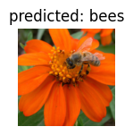
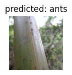
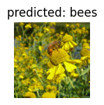
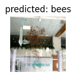
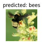
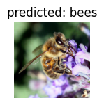
Let’s now visualize the inference of the trained model on some sample images from the validation step

[11]:

def visualize_model(model, num_images=6):
    was_training = tf.keras.backend.learning_phase() == 1
    images_so_far = 0
    fig = plt.figure()

    for i, (inputs, labels) in enumerate(dataloaders['val']):
        inputs = tf.convert_to_tensor(inputs.detach().numpy())
        labels = tf.convert_to_tensor(labels.detach().numpy())

        outputs = model(inputs, training=False)
        preds = tf.argmax(outputs, 1)

        for j in range(inputs.shape[0]):
            images_so_far += 1
            ax = plt.subplot(num_images//2, 2, images_so_far)
            ax.axis('off')
            try:
                ax.set_title(f'predicted: {class_names[preds[j]]}')
            except:
                continue
            imshow(inputs[j])

            if images_so_far == num_images:
                model(inputs, training=was_training)
                return

    model(inputs, training=was_training)

[13]:

visualize_model(transpiled_model)

../../_images/demos_examples_and_demos_resnet_to_tensorflow_28_0.png

../../_images/demos_examples_and_demos_resnet_to_tensorflow_28_1.png

../../_images/demos_examples_and_demos_resnet_to_tensorflow_28_2.png

../../_images/demos_examples_and_demos_resnet_to_tensorflow_28_3.png

../../_images/demos_examples_and_demos_resnet_to_tensorflow_28_4.png

../../_images/demos_examples_and_demos_resnet_to_tensorflow_28_5.png

Conclusion#

We’ve just seen how the transpiler can be used to convert a model from PyTorch to TensorFlow and train the converted model in TensorFlow.

Head over to the tutorials section in our documentation if you’d like to explore other demos like this. You can also run demos locally on your own machine by signing up to get a transpiler API key for local development.

If you have any questions or suggestions for other interesting demos you’d like to see, feel free to ask on our Discord community server, we look forward to seeing you there!